Home Science Page Data Stream Momentum Directionals Root Beings The Experiment
We have derived the above general equation for directionals, Equations 18->20. We now apply it to specific instances beginning with P=0. We get the Fractal Root Pattern when P=0. This was expected (see page 4 Section II). This equation is at the root of all that follows, replicated in strange patterns, divisions and differences, yielding a marvelous complexity that inevitably folds up into a ... But we're getting ahead of ourselves. Below is the Fractal Root Equation in all its simplicity, elegant in its framing, awesome in its description of the inward spiral of the Decay of Experience with Time. The whole potential is included within all of the Decaying Parts. No part ever disappears altogether and yet diminishes rapidly. The parts act in concert to achieve a larger effect. The individual parts quickly fade into obscurity while their accumulating footprints remain. The Path more traveled becomes a Road.
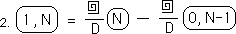
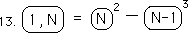
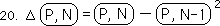
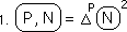
We now apply Equation 18, when P = 1.
Substituting the expression from Equation 1, we get the equation below. Notice that the first Directional is written as a function of raw data alone, for the first time. We'll get back to that.
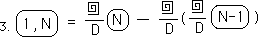
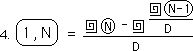
Rewriting the above Equation:
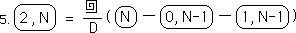
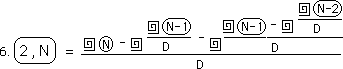
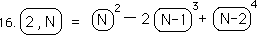
We now apply Equation 20, when P = 2.
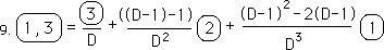
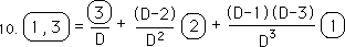
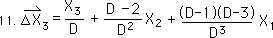
Substituting the appropriate expressions and rewriting, we get the following equation. Notice that the 2nd Directional is written finally in terms of the data only. Notice also the emerging Fractal pattern in the Equation itself. The first term is replicated in the second, while the first two terms are replicated in the third term.
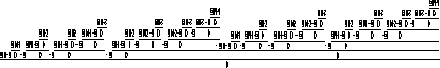
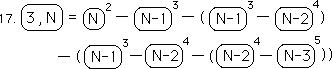
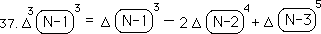
We now apply Equation 20, when P = 3.
We substitute in the appropriate expressions from the above derivations and rewrite the equation in the same style as above. Again notice that the 3rd Directional is written as a function of the raw data, alone, no intermediate steps or expressions. Of course the number of unfurling expressions are doubling each time. Also the fractal pattern continues with the fourth expression. It contains the first three expressions, each of which contains the expressions before. The equation size doubles each time. This time it had to be squeezed onto the page.
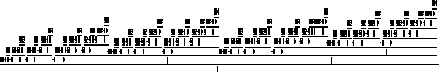
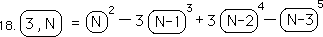
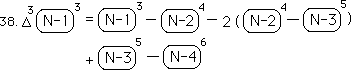
We now apply Equation 20, when P = 4.
We substitute in the appropriate expressions from the above derivations and rewrite the equation in the same style as above. The 4th Directional is written as a function of the raw data, alone, no intermediate steps or expressions. The fractal pattern continues with the fifth expression. It contains the first four expressions, each of which contains the expressions before. It is quite evident that this equation, which is a fractal itself, describes a fractal phenomenon, replicating itself upon small and large levels. It is the fifth element of the Fractal Function Set, the first element when P=0.
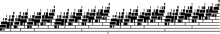
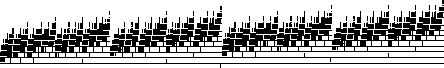
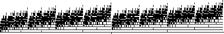
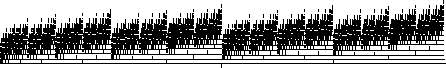
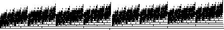
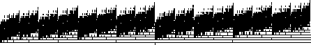
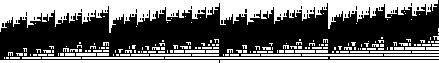
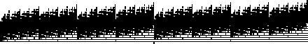
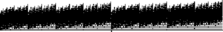
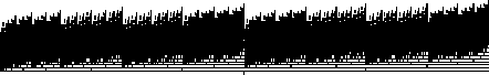
Following are some examples of more Fractal Equations from the Fractal Function Set. Although mostly illegible, they reflect the fractal nature of the equations.
Below is an animation of the fractal function set from P=0 through P=18. The purpose is only to illustrate the fractal nature of the equation itself when viewed over time. With each individual frame the equation is doubled or halved depending upon which way the animation is viewed. Notice how each equation bears an incredible similarity to the last although they've been shrunk or expanded.
{Only on Mathematica}
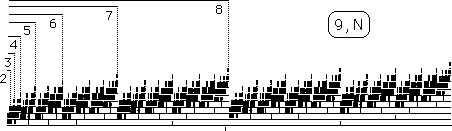
To give an idea of how packed this equation is for P=18, we present the levels of compression. The part of the equation under the line associated with 17 is when P=17. The smallest line, when P=11, is only 4 pixels wide. Consequently the part of the equation when P=9 is only 1 pixel wide.
The equation below is an expansion of that one pixel width in the above equation, i.e., when P=9. It is still an illegible equation. Look at the size of the equation when P=4. This was the last legible equation (see above) and it was really crunched. The single pixel on the far left represents the Fractal Root Equation.
The above equations, from P=0 through P=18, are examples of furled equations. The last general equation that was unfurled was the expression for the F function for the Decaying Average in Section I, page 6. All the rest of the general equations have been furled so that they would fit upon the page. Of course the individual expressions derived above for the First Directional, when N=0->3, are all unfurled expressions, Section I, pages 11 & 12. As seen above, even furling the equations does not help much when P>4. We need to abbreviate these equations even further if we are to ever find the H function for all Directionals. As a matter of fact the number of furled expressions in any of these furled equations equals 2P and these include many expressions that need to be unfurled more than once.
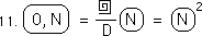
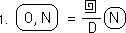
Let us ravel our functions into some simpler expressions. We will be employing the circle function as defined in the Unraveling section in Equation 5, Section II, as the Unfurling function divided by D. The exponent for the circled Data will be the number of times the circle function is used plus 1, the original circle. So in the first example below we ravel our furled equation once, so our exponent on the circled N is two, consistent with the previous results (equation 15, Section II, Page 12 of the Unraveling section).
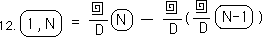
Repeating Equation 3 above for the First Directional.
We ravel it in the manner prescribed above. This yields the following raveled expression.
This is the elusive G function for the 1st Directional that evaded us in the more specific approach.
We apply the same raveling techniques to Equation 6 above and get the following equation.
Combining terms we get this intriguing expression for the 2nd Directional. Note that it is a furled and raveled equation in terms of Raw Data only. There are no derivatives in the equation.
We apply the same raveling techniques to the furled equation for the 3rd Directional, Equation 8 above, and get the following equation.
Combining terms we get the following expression. The coefficients are sneakily like the coefficients for the Binomial Theorem.
Finally we apply the same multiple raveling techniques to the furled equation for the 4th Directional, Equation 10 above. We combine terms and get the following equation. Again we get the Binomial Coefficients with alternating signs.
These furled and raveled equations are more concise expressions of the early Directionals. We have finally got the elusive G function for the First Directional. Further the general expressions for the 2nd through 4th directionals fell easily out through this raveling technique. But we now introduce one more reduction function, the Folding Function.
We are not going to delve into the meaning of the Folding Function for the time being. We are going to simply define it. It is related to a Delta function. A Delta function is based on change, which is based upon differences. All the derivatives in Physics are Delta functions because they are based upon change. All the derivatives of the Data Stream are Delta functions, because they, too, are based upon differences. In some ways the Folding Function is a meta-Delta function. The simplest expression of the Folding Function is in the first equation below. Notice that the P is unaffected. Folding, in this first case, means to convert from Directional form to Delta Form. Unfolding means to convert from Delta Form to Directional Form.
The 2nd Definition of Folding is a little more general. It defines what to do with higher powers of Folding. It continues the pattern established above. The Folding exponent is reduced by one when the expression is unfolded and increased by one when it is folded back up.
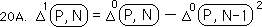
Here is Equation 20 expressed with exponents, after the style of Equation 21.
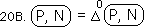
The zeroth power of the Folding Function is the general Directional itself. The style is similar to previous results, where the zeroth power turns the expression into another form. Remember that the zeroth power of the Raveling Function for the Decaying Average is the raw Data.
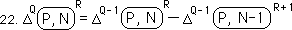
The 3rd Definition of the Folding Function is the most general. While the previous two definitions assumed that the exponent for the Raveling Function, the Circle Function, was either 1 or 2, this definition acknowledges that, in general, the exponents will be R and R+1. When the function unfolds, the level of Raveling increases and the level of Folding decreases. When the expression Folds up the level of Folding increases and the level of Raveling decreases.
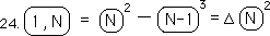
Below is the general expression for the 1st Directional, Equation 21 in the Unfurling Section, folded up once according to the definition of Folding.
In a similar way we fold up the raveled equation for the first Directional, equation 13 above. This is another expression of the G function. It is a furled, raveled and now folded expression in terms of the raw Data only. If this expression is unfolded, unraveled and unfurled according to these rules, then we get an equation that only contains the raw data with the basic operations of addition, multiplication and their inverse functions.
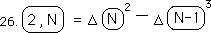
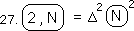
Below is the Raveled expression for the 2nd Directional, equation 15 above.
We first fold up the two halves of the expression
We then fold them up again. Below is a folded, raveled, furled expression for the 2nd directional, in terms of the raw Data only. In order to evaluate the expression, it must be unfolded, unraveled and unfurled.
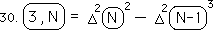
Below is the raveled expression for the 3rd Directional, Equation 17 above.
We fold up the four pairs of raveled expressions once.
We now fold up these four folded expressions.
On the third fold, we fold these two doubly folded expressions into one expression.
The general expression for the third directional could be stated as the triple folding of doubly raveled raw data. The 2nd directional is the double folding of the doubly raveled raw data. The 1st directional is the single folding of the doubly raveled raw data. The zeroth directional, the Decaying Average, is the zeroth folding of the doubly raveled raw data. In other words the Decaying Average is the doubly raveled raw data. A pattern is emerging. Let us look to see if the fourth directional is the quadruple folding of the doubly raveled raw data. To discover this we will unfold this expression.
This is the expression after the first unfolding.
The first expression is the 3rd Directional. Below is its unfolded but raveled expression, equation 29 above.
This is the 2nd expression of Equation 33 unfolded again.
We then unfold these two expressions once more. Now these four expressions are only folded up once.
We combine terms.
We then unfold these three terms for the last time, with the following raveled, but unfolded result.
We combine terms.
We then subtract the above equation from equation 34 – ala equation 33, and obtain the following Raveled expression for the 4th directional. This is the same expression as equation 19 above, confirming our hypothesis that the fourth unfolding of the doubly raveled raw data is the fourth directional.
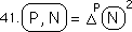
This leads to the following result. The Pth directional is equal to the doubly raveled data folded up P times. We call this the Seed Equation for the General Directional. It is a simple concise equation for the general Directional written in terms of the raw data alone. It has been demonstrated but not proved.
This is the H function for the general directional that we proved existed in the first section of this notebook. Our reductionist approach succeeded. Who needs a contextual approach, when our content-based approach leads to such simplicity?
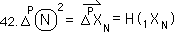
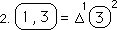
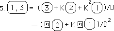
Before dealing with the above question, let us test our Seed equation, when P = 1 and N = 3. This is the Seed Equation.
This is the Seed Equation when P = 1 and N = 3. Such a simple expression.
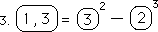
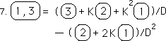
We unfold the expression once.
We then unravel the first expression once and the second expression twice.
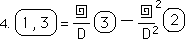
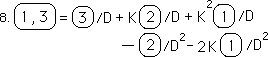
We then unfurl both expressions once. The first of the expressions turns into raw data. The second expression must be unfurled again.
We unfurl the second part of the expression for the second time, reducing it to an expression of raw data.
We put this expression back into Equation 5.
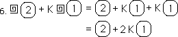
We multiply through to remove the parenthesis.
We then convert the constant K to its D form, (D-1)/D, and combine like terms.
Finally we simplify the expression.
Writing it in a more familiar form we find that it is the same equation that we derived in Part I, Section 4, page 12. Hence it verifies our Seed equation.
Let it be pointed out that this is only the third Data Point of our 1st Directional. Our feet are barely getting wet with the data and on such an elementary level, the 1st Directional only, and still the Seed Equation needed to be unfolded once, unraveled twice, and unfurled twice, to get a workable expression, in terms of the raw data alone.